Forward-Looking Cycle Time Metrics

It’s simple enough to measure the cycle time for lots after they ship, both on an individual and an aggregated basis. But what we would also like to know is, based on current performance, what will the cycle time be for lots that are still in the fab? At the individual lot level, this information can be helpful in predicting which lots will be on time (and which will not). At a higher level, understanding the fab’s expected cycle time for lots currently in process can be useful for setting delivery dates for new orders. This information can also give us an early warning of cycle time problems during an upturn (and there will always be one coming eventually), so that we can make operational changes before cycle time and WIP levels become unacceptably high. In this article, we review several forward-looking cycle time metrics. We also propose a new metric for predicting the future cycle time of lots in the fab, based on an extension to WIP Turns.

There are two general ways of predicting an individual lot’s future cycle time in a fab. One method involves using discrete event simulation. A simulation model can incorporate tool downtimes, operator constraints, current WIP levels, etc. Simulation models require very detailed data to be accurate, however, particularly regarding tool downtimes. Maintaining such detailed models has proven impractical for most fabs. 

The second, much simpler, method involves using static projections based on planned cycle time data for each step. Static lot shipment projection is a matter of storing a planned cycle time number for each route-step combination for all routes in the fab. At any point, we can add up those planned cycle times for all future steps for a given lot, add that total time to the current time, and get an estimate of when we think that this lot will complete. We can aggregate this data across lots and use it to predict the number of lots that will ship on a given day, or that will arrive at a key tool or operation within a given timeframe. This is what we do in the FabTime reporting module.

There are some implementation issues to consider with this method. Chief among these is that we need to have access to the planned cycle time data for each step. What we often see people do here is use a planned process time per step and multiply that by a target x-factor that may vary for each route. That x-factor may also be adjusted on the fly to reflect changes in lot priority. Sometimes historical data is also used here. 

The primary issue with this method of forecasting individual lot shipment dates using planned cycle times, however, is that it doesn’t typically take current fab performance into account. The method is only as good as the quality of the planned step cycle times, and what’s realistic there can change depending upon fab conditions. Fortunately, there are several forward-looking metrics that we can use to predict aggregate future cycle time performance based on current fab conditions. Once we have a better estimate of the overall cycle time performance for lots in the fab, we can convert that that to an expected x-factor and use it to refine the forecasts for the individual lot completion dates. Let’s discuss those forward-looking aggregate metrics in turn.

A forward-looking metric that has long been included in FabTime is Dynamic X-Factor. Dynamic x-factor is a point-in-time metric that is recorded frequently (e.g., every hour) as Total WIP / (Non-rework, non-hold WIP running on tools). It can be shown that in the long run, the average of a series of dynamic x-factor observations will be equivalent to the shipped lot x-factor, meaning that it can be used to predict future cycle times based on current performance. Dynamic x-factor is intuitive and easy to calculate and also gives us a window into short-term periodic. It’s also easy to filter dynamic x-factor by product, route, or priority, to estimate the future x-factor for different types of lots, as shown in the figure below. The chart on the left shows the overall dynamic x-factor for the fab. The one in the middle shows a low-volume, higher priority product, while the one on the right shows a lower priority product (with a consequently higher x-factor).

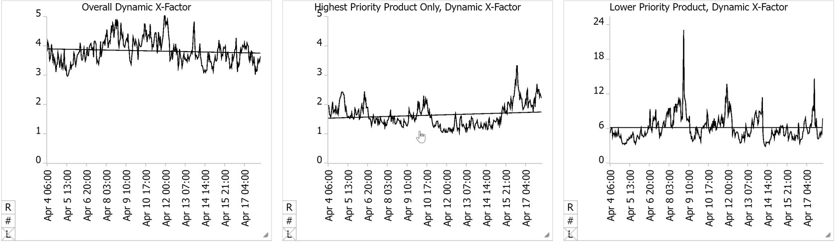
We know of several fabs that use dynamic x-factor in a control chart-like fashion, by which they take note if it drifts upward, outside of normal fluctuations. These fabs also use dynamic x-factor to highlight short-term, periodic effects in the fab, such as shift change. On a short-term basis, we can’t necessarily look at the graph of our fab-wide dynamic x-factor and expect it to exactly track with future shipped lot cycle time values on a particular date. The two primary reasons for this are: 

1. Product mix changes combined with the time lag between dynamic x-factor and x-factor make short-term comparisons difficult; and 
2. Systematic issues in how we measure and report theoretical cycle time, and how we log transactions in the MES, can lead to differences in the reported values for the two metrics. For example, do we have good data on whether lots are in process or not? Are there lots on extended hold that are inflating dynamic x-factor relative to shipped lot cycle times?

It’s also necessary to decide what time frame to use to take an average dynamic x-factor value as a forward cycle time estimate. We recommend using at least a week of data, possibly longer for low-volume products with more lot-to-lot variation.

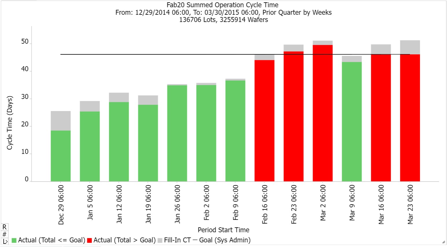
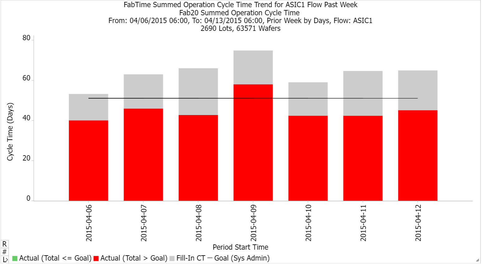
Another forward-looking cycle time metric that we coded into FabTime at the request of a customer is Summed Operation Cycle Time. The summed operation cycle time chart predicts cycle time based on current operation-level cycle times and, for operations that have not been recently completed, planned cycle times. Operation-level cycle times are estimated and then summed to provide an overall cycle time estimate, which we can pareto by area, operation, tool-group, segment, etc. This is a slightly higher-level, and more forward-looking approach than simply looking at actual operationlevel cycle times. It says, based on our current performance and our planned performance, here’s what we can expect our future cycle time to be, if the current situation continues. In the example to the right, we can see a worrying increase in the weekly Summed Operation Cycle Time over the course of the quarter.

Complexities to using this metric include the following:

• If we drill down to look at summed operation cycle time by operation, we cannot simply add up the resulting total summed operation cycle times to get the overall average summed operation cycle times, unless each operation is represented by the same number of wafer moves on each flow. This metric is intended to summarize at the flow level first, and then perform a weighted average across flows. If operations are not represented evenly on all flows, then there is no reason for the operation-level summed operation cycle times to add up to the total summed operation cycle time across all flows. This can make analyzing the results confusing.
• As with the individual lot projection method discussed above, we need planned cycle times by step to fill in for operations that haven’t been recently completed. Depending on a fab’s situation, there can be so much fill-in data that the charts are not useful. Seeing considerable fill in cycle time data, as in the example below, can make this chart non-intuitive or implausible to users.

WIP turns can be used to get a forward estimate of cycle time. 

Turns = Moves / Average WIP

By default, FabTime scales raw turns to turns per day, with scaled turns = (raw turns) * 24 / (chart length in hours). WIP turns tell us, on average, how many times per day the fab is moving each wafer. If we also know the average number of steps that each wafer goes through, then we can predict the average cycle time for our current WIP by taking:

(Average Steps in a Flow) / Turns, where Turns = Steps per Wafer per Day

For example, if we move each wafer 8 times per day on average, and each wafer requires 400 steps to complete processing, on average, then our cycle time will be 400 steps / 8 steps/day = 50 days. 

Of course, the number of steps used for this calculation must be consistent with the level at which we are tracking moves. If this is the case, and if we maintain a consistent turns rate, then we can expect average cycle times in the future to be about 50 days. 

The tricky part of using WIP turns to predict overall average fab cycle time lies in knowing the right number of steps to use in the calculation. What you need for the overall average is a weighted average number of steps, where the weighting is by relative proportion of WIP. Because product mix in a fab can change rapidly, the weighted average number of steps may change, too, particularly if you have process flows that vary in complexity. 

We have previously recommended that you not get too hung up on keeping track of this on a daily basis as your mix changes, but to perhaps keep a spreadsheet in which you track the number of steps per major flow. However, in thinking about that more recently, we would like to suggest another solution.

Our new proposal is that instead of trying to maintain a weighted average of number of steps per flow in the constantly changing environment of the fab, we instead include the number of steps per flow as an attribute of each lot. With this data, for any turns chart we could also sum up the number of steps in the flow across all WIP included on the chart, and then divide by the number of lots. In this way, we would generate a relevant forward estimate of cycle time for whatever WIP was selected, based on how that WIP was moved over the chart’s time period.

We initially called this metric Turns-Predicted Cycle Time, but later renamed it, at the request of a customer, to the simpler Dynamic Cycle Time. There remains some complexity in getting the number of steps on a flow, given differences in what different fabs consider steps. It should be possible to estimate the number of steps on a flow by looking at the historical number of moves for shipped lots. Because turns are calculated as moves / WIP, if we use the number of moves for shipped lots, this will give us an apples-to-apples number for estimating total cycle time from turns. Of course, this will be more difficult for brand new flows with no shipped lots. However, we believe that fabs will probably have some way to estimate the number of steps per flow that could be included as an attribute for new lots. 

For example, suppose that we have three 25-wafer lots. One follows a 300-step flow, one a 400-step flow, and one a 500-step flow. We can compute an average number of steps per wafer as 400. 

Now suppose on a given day we have 750 wafer moves. The turns rate is moves / WIP = 750 / (3*25) = 750/75 = 10 moves/day. The dynamic cycle time estimate would be 400 steps / 10 moves/day = 40 days. (Provided, again, that steps are equivalent to the recorded moves.) Being based on the turns rate, this metric should tick upward quite quickly if the fab starts to either build WIP or slow down in terms of total moves.

We can use dynamic x-factor, summed operation cycle time, or dynamic cycle time to predict average future cycle times for the fab as a whole, and (probably with more accuracy) for individual products. If we want to use any of these projections to make decisions or commitments based on the information, we should of course first validate the predictions against actual performance. This will help to identify systemic issues that may be biasing a given metric high or low. Once a given metric is validated, it can be used at a high level to influence future commit dates and to anticipate problems in the fab (e.g., we need more capacity or staff to avoid unacceptable cycle times). If we want to use this data to refine forecast completion dates for individual lots, then we’ll need to follow a process like this. For dynamic x-factor:

1. Estimate average dynamic x-factor for a route and priority class of interest based on, for example, this week’s performance. 
2. Use that projected x-factor as a multiplier of future step process time estimates to predict individual lot completion dates. This may be more accurate than simply using the planned cycle times by step, as outlined above.

 For summed operation cycle time or dynamic cycle time, we need one extra step: 

1. Estimate overall cycle time for a route and priority class of interest based, for example, this week’s performance. 
2. Convert that overall cycle time into a predicted x-factor by dividing by theoretical cycle time. 3. Use that predicted x-factor as in Step 2 above.

Forward-looking cycle time metrics are useful for predicting which lots are likely to be late (and adjusting accordingly if possible), for setting commitment dates for future starts, and in general for understanding when cycle time is likely to increase, so that corrective action can be taken. In this article we have discussed a general method for forecasting shipment dates for individual lots, and then reviewed several metrics for predicting future cycle time x-factors and shipped lot cycle times. We have also introduced a new metric for forward-looking cycle time based on the WIP turns rate and the total number of steps per lot. We have implemented Dynamic Cycle Time in the FabTime reporting module, and hope that all of you will find it useful.