Improve Fab Cycle Time by Tracking the Right Equipment Reliability Metrics
Well-chosen equipment reliability metrics can help communication between fabs and equipment suppliers and drive cycle time improvement

When asked to name the factors that contribute the most to cycle time in their fabs, people give a range of responses. They might mention bottlenecks or product mix or time constraints between process steps. But far and away the most common response is: equipment downtime.
This is not to hand out blame to equipment vendors. (INFICON sells a range of sensors that are used in semiconductor equipment.) Cutting edge wafer fabs are constantly pushing the boundaries of technology, meaning that fabs are using leading edge tools that may not yet have all the kinks worked out. Older fabs, in contrast, struggle with equipment that has been in use for many years and may not be as widely supported as it once was. This is not to blame fab maintenance technicians, either, for the same reasons. Maintenance techs also suffer from the common challenge of not being able to be in two places at one time, which is hardly their fault.
What we think IS partially to blame is a lack of understanding about which equipment reliability metrics, if improved, would be most helpful in reducing fab cycle time. People track mean time between failures (MTBF) relentlessly. But MTBF is almost meaningless for cycle time improvement. People track OEE on all the tools, even though OEE in its default formulation is not relevant for non-bottleneck tools (though certain OEE loss factors remain helpful). Fabs pressure equipment suppliers to deliver better equipment reliability. But it’s not clear that everyone involved has the same understanding of what “better equipment reliability” means.
What’s meaningful for cycle time in terms of equipment reliability are four things:
- Overall availability
- Duration of unavailable time, measured as mean time to repair (MTTR) and/or green-to-green time
- Repair time variability
- Availability variability
In this article, we explore why these four aspects of equipment downtime drive cycle time and propose associated metrics and actions to improve them. It is our hope that fab personnel, especially maintenance engineers, as well as equipment suppliers will find this article a helpful reference to improve understanding of and communication about equipment reliability.
How downtime affects cycle time: definitions
Downtime hurts cycle time by degrading each of the three fundamental drivers of cycle time: utilization, variability and number of qualified tools. See Fundamental Drivers of Wafer Fab Cycle Time for an overview of how these factors impact cycle time in general. Here, we’ll talk about each of these, in turn, in the specific context of equipment downtime.
First, a few definitions:
Manufacturing Utilization of a tool is the ratio of productive time to manufacturing time, where manufacturing time is the total time that the tool is available to manufacturing to process wafers. This definition is from the SEMI E10 Specification for Definition and Measurement of Equipment Reliability, Availability, and Maintainability (RAM), which classifies the tool states as shown below.

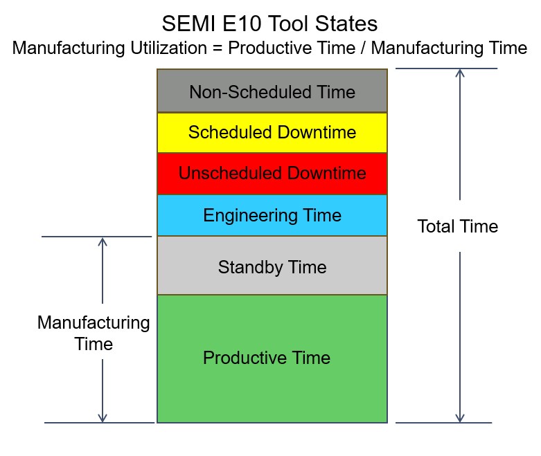
We have: Utilization = Productive Time / Manufacturing Time
= Productive Time / (Productive Time + Standby Time)
In general, as standby time gets small, utilization becomes high. With no standby time, utilization will equal 100%. With no productive time, utilization will equal zero.
X-Factor is a metric for tracking cycle time, recorded as total cycle time / theoretical (best case) cycle time. X-factor can be measured at the factory level or at the operation level. When measured at the operation level, it typically includes all time from when the lot moves out of the prior step until it moves out of the current step, including travel time, queue time, and process time.
An Operating Curve is a graph that shows cycle time x-factor on the y-axis and utilization on the x-axis. Operating curves are used to show the impact of utilization and other factors on x-factor.
The operating curve for a one-of-a-kind tool, under certain assumptions, follows this formula:
Cycle Time X-Factor = 1 + [Utilization/(1 – Utilization)]*(Variability Factor)
What this formula means is that as utilization approaches 100%, in the presence of any variability, cycle time gets very high. Only when the variability factor is zero is cycle time x-factor equal to one (no queue time).
When the variability factor is equal to one, the equation for x-factor reduces to a simpler form:
Cycle Time X-Factor = 1 / (1 – Utilization)
This equation shows that as utilization approaches 100%, we have one divided by zero, which approaches infinity. Of course, we don’t have infinite cycle time in practice because we don’t have infinite WIP. But what these equations illustrate is that we need for there to be at least some standby time to achieve good cycle time. Now let’s look at how downtime affects utilization (and hence cycle time).
Downtime increases utilization by taking away standby time
We can see from the above definitions, particularly from the schematic of the E10 Tool States, how downtime impacts utilization. When productive time is held constant, both scheduled and unscheduled downtimes reduce standby time, thus increasing utilization. Increasing utilization in turn increases cycle time.
Let’s look at an example. Suppose we have a tool with combined scheduled and unscheduled downtime of 16.8 hours per week (10% of total time), no engineering time, and no non-scheduled time. This puts us on the red operating curve shown to the right, where we hit 100% utilization when the tool is run 151.2 hours per week (168 hours – 16.8 hours).

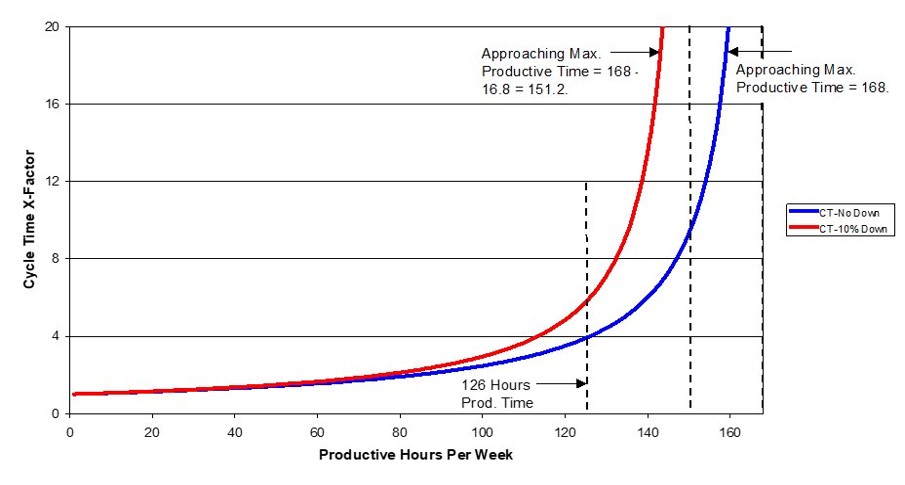
As productive time approaches 151.2 hours per week (the rightmost part of the red curve), cycle time gets very high. If the actual productive time in a week is 126 hours, then the standby time will be 151.2 – 126 = 25.2 hours, and we’ll have:
Utilization = 126 hours / 151.2 hours = 83.33%
Following the simple formula for x-factor, we have:
X-Factor = 1 / (1 - .8333) = 6X
But, now suppose we can convert the 16.8 hours per week of equipment downtime to standby time. What this does is push out from the red curve to the blue curve, where 100% utilization is reached when the tool is run 168 hours per week. If we have the same 126 hours per week of productive time as in the example above, we’ll have 168 – 126 = 42 hours of standby time, and our effective utilization will drop to 126 / 168 = 75%. If we once again follow the simple formula for x-factor, we will have:
1 / (1 – Utilization) = 1 / (1 - .75) = 4X.
That is, converting 16.8 hours of downtime (10%) into standby time reduces the average cycle time by ~33%, from 6X to 4X. Because the operating curve is non-linear, the closer we are to the steep part of the curve, the greater the impact will be from converting downtime into standby time.
Any hours (or even minutes) of scheduled or unscheduled downtime that can be converted to standby time increase the tool’s buffer capacity and keep it away from the steep part of the operating curve.
What does this mean in terms of metrics that capture the impact of downtime on utilization?
Equipment engineers can support cycle time improvement by ensuring that tools have the highest possible availability (the lowest possible amount of combined scheduled and unscheduled downtime), on a day-to-day and week-to-week basis.
Now, let’s consider variability.


Want to learn more about cycle time drivers in your fab?
Variability from downtime changes the shape of the operating curve
Variability changes the shape of the operating curve. Remember that our formula for the operating curve for a one-of-a-kind tool as shared above was:
Cycle Time X-Factor = 1 + [Utilization/(1 – Utilization)]*(Variability Factor)
The formula for the Variability Factor is: (CVa2/2) + (CVp2/2), where CVa is the coefficient of variation of time between arrivals and CVp is the coefficient of variation of the process times.
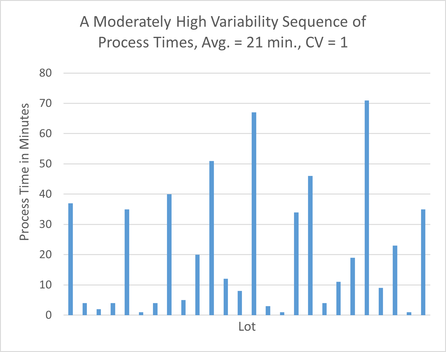
Coefficient of variation is a statistical measure that records how far things are away from the average. A series of values that are all the same would have a coefficient of variation of zero, while a higher variability set of values might have CV= 1, as shown in the example below. What the formula for x-factor shows is that the higher the variability factor, the higher the cycle time. And the higher the utilization, the greater the impact of the variability factor.

There’s a more detailed formula for the operating curve that we have coded into our Operating Curve Spreadsheet. That formula includes multiple tools, batch arrivals, and hot lots. It also includes an approximation for a single downtime distribution.
We will spare you the full complexity of the formula (see the CT Calculator Details sheet of the spreadsheet for more information), but what’s relevant here is that it replaces CVp2 (the base coefficient of variation of process times) in the variability factor with a calculated system variation value that includes the impact of equipment downtime on the effective process time experienced by each lot. The relevant portion of that formula for looking at downtime is this term, which is added to the base process time variability:
Downtime Variability = [Availability*(1 – Availability)] * (MTTR/Avg. Process Time) * (1 + CVr2)
Where CVr is the coefficient of variation of the repair time and Availability = 1 – Percent Downtime.
Availability: Let’s look first at availability. If availability is perfect (100%), then the first term becomes zero, and the entire Downtime Variability term is zeroed out. Otherwise, the first term is maximized (i.e., has the most impact) if availability is 50%. Then [Availability*(1 – Availability)] = .5*.5 = .25. The availability value thus has a relatively low impact here, though of course overall availability has a major impact on the utilization effect of downtime, as described above.
What’s clear when we look at this formula is that both MTTR and CVr can have a significant impact on cycle time.
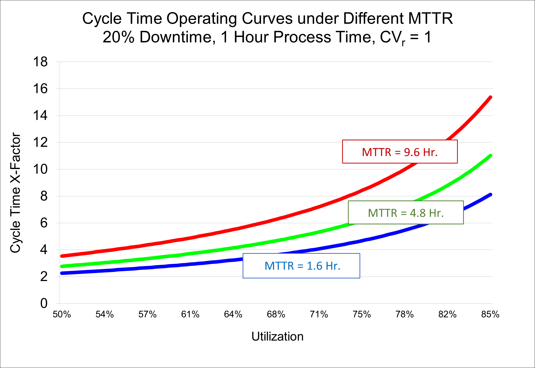
Repair Time Duration: Let’s look at the middle term of the downtime variability equation: MTTR/Average Process Time. The longer the repair time (MTTR), the greater the impact on cycle time. This reflects what people see in the fab. It’s the long downtimes that really hurt productivity. Large amounts of WIP pile up, and it can take a long time to recover from these occurrences. This is especially a problem for one-of-a-kind tools, but applies to tool groups with multiple tools, too. The impact is particularly significant for tools with short process times, because more lots are impacted by the downtime.
An example from the Operating Curve Spreadsheet is shown below, where MTTR varies, while the total percentage downtime is held constant. For the same total amount of downtime, a longer, less frequent repair time has a much more negative impact on the operating curve than a shorter, more frequent repair time. See Issue 22.01 for a discussion of the implications of this behavior on PM scheduling.

Repair Time Variability:
Let’s look at the last term from the Downtime Variability equation: (1 + CVr2). When the coefficient of variation of the repair time is zero, that means that the repair always takes the same amount of time. This is the best case for variability reduction and hence, for cycle time. Anything greater than zero drives up the impact. And because CVr is squared, the impact becomes particularly large when CVr is greater than one. This reflects what we see in the fab – when repair times are highly variable, this means that some of them are long. And again, those long repair times are the ones that have the most significant impact on cycle time.
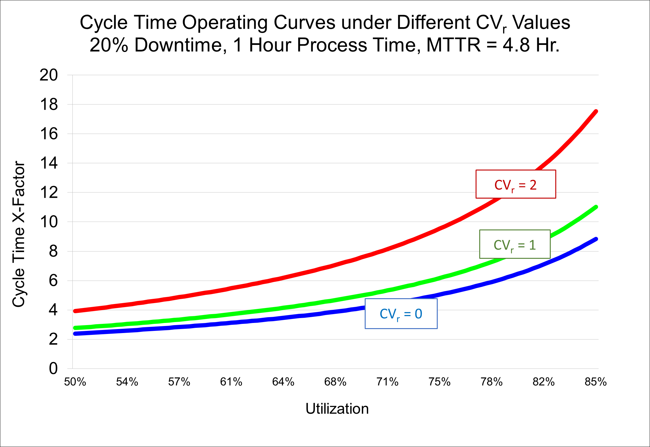
Looking at another example using the Operating Curve Spreadsheet, again with 20% downtime, consider below varying the coefficient of variation of the repair time (where the average repair duration is 4.8 hours). The blue line shows constant repair times, while the green and especially the red show greater repair time variability. Because CVr is squared in the formulas, the red line looks especially bad. This high level of variability can be realistic, however, when we consider something like a possible three-day downtime while the maintenance team waits for a part to arrive from the equipment supplier.

What does this mean in terms of metrics that capture the impact of downtime on variability?
Equipment engineers should track the average duration of unavailable time (MTTR), broken out into scheduled vs. unscheduled downtime. They should also keep an eye on the maximum repair times and strive always to reduce those. Tracking each period of unscheduled downtime according to how the time was spent (e.g. waiting for a technician vs. waiting for parts) is also useful here. This information, aggregated across like tools, can give insight into needed training for maintenance teams, which spare parts contracts are worth investing in, etc.
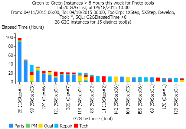
Green-to-green time (G2G) is also a useful metric here. G2G measures the total elapsed time between two good states (standby or productive), grouping together scheduled and unscheduled downtime, qual time, etc., as shown below. The idea is to look at the total time that the tool is unavailable to manufacturing, because this is the factor that most directly drives up cycle time.

Equipment engineers should track the coefficient of variation of both scheduled and unscheduled downtime events by tool group and strive to reduce those. Note that the CV can be reduced in part by focusing on bringing in outliers in the MTTR, as described above. It may also be useful to track the CV of Green-to-Green instances for a tool group, and try to reduce that. MTTR, G2G, hours of unscheduled downtime by sub-state, and CVr for scheduled and unscheduled downtime are all standard charts in the FabTime reporting engine.
What about Mean Time Between Failures (MTBF)?
What we’ve seen in this section is that average downtime duration as well as the variability of the downtime duration have a significant (and distinct) impact on equipment cycle time. Increasing mean time between failures, on the other hand, won’t improve cycle time, except as it drives overall availability, and can sometimes be counterproductive. For the same downtime duration, sure, it’s better if the tool goes down less frequently. But, it’s also better to bring the tool down regularly for maintenance than to risk a long unscheduled downtime. And it’s better to bring the tool back up right away after a downtime to work off the WIP that has accumulated, even if it means bringing the tool down sooner for the next PM (vs. doing the PM while the tool is already down).
Downtime makes the number of qualified tools more variable
The third fundamental driver of cycle time at the tool group level is the number of qualified tools. See Issue 20.05: The Impact of Tool Qualification on Cycle Time for more details. The number of qualified tools for a given recipe has a significant impact on cycle time, particularly as we go from one qualified tool to two. There’s about a 50% reduction in cycle time when going from one tool to two (at the same utilization for each tool), with about another 25% reduction achieved in going to three qualified tools, and effects diminishing beyond that, as shown below.


This behavior occurs in the presence of any type of variability and is not specific to equipment downtime. However, it’s easy to see that downtime reduces the number of qualified tools that are available at any given time. Sometimes, downtime reduces the number of available qualified tools to zero, which is the worst case for cycle time.
The impact of downtime on number of qualified tools is captured, at least indirectly, by tracking the coefficient of variation of the availability of each tool. Consider the sequence of availability values recorded for each shift for a tool over a one-month period. The best case for cycle time is, of course, for that sequence to consist of all values of 100%. But if the average availability of the tool is, say, 90%, then the best case for cycle time is for each tool to be available for 90% of each shift, day in and day out, down for only 1.2 hours out of the 12-hour shift. (Barring very long qual times, at least.)
The worst case for cycle time is for the availability to sometimes be 100%, but sometimes be 0% (down for the whole shift, or, even worse, for days at a time). This is also the sequence that will give us the highest coefficient of variation. Remember, CV measures how widely things are dispersed from an average.
What happens when we have individual tools with a high CV of availability is that we have a higher likelihood of having multiple tools unavailable at the same time, and thus of having lots arrive to find no qualified tools available, or to find only one qualified tool available when there should have been redundancy. That’s what’s happening in the chart below, which shows a spike in per visit cycle time for a tool group that theoretically has four qualified tools, but also has high availability variability.

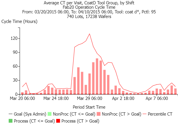
The average availability for each CoatD tool over a three-week period is 60% and the average utilization of available time is 81.4%. The CV of availability for each tool in the tool group over the three-week period (measuring availability by 12-hour shifts) ranges from 0.58 to 0.67.
When we look at the average cycle time per visit through this tool group in the chart on the previous page, we see that it is highly variable. Note the period between March 29th and April 1st, when the per visit cycle time reaches as high as 3.2 days, relative to a process time of only 1.3 hours. The x-factor is 58 for the worst shift.
One reason that the cycle time is so high during that period is that two of the four tools in the group were completely unavailable for two full days at the same time. What we want when we look at availability by shift is for the values to be consistently high, not sometimes high, but often zero. When availability is highly variable, our chances of having too few tools available to process incoming WIP are high.
What does this mean in terms of metrics that capture the impact of downtime on number of qualified tools?
Equipment engineers should track the coefficient of variation of availability for each tool by recording availability per shift (or per day), and then calculating CV as standard deviation / average of those values.
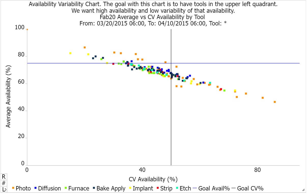
A useful chart that we include in the FabTime reporting module shows Average vs. CV of Availability by tool as a quadrant chart. An example is shown below. Each dot represents an individual tool, and the tools are colored according to their area in the fab. In this example, the worst-performing tools are the ones in the lower right-hand quadrant. These tools have poor availability and highly variable availability. We can never count on having the tool be up and running. The tools in the lower right-hand quadrant should be the focus of equipment reliability improvement efforts.

Another metric that focuses on availability variability is A20/A80. A20/A80 generates the sequence of availability values by day or shift and identifies the availability achieved in the best 20% of the shifts and the best 80% of the shifts. When those values are close together, that means that the availability is consistent from shift to shift.
In summary, what metrics should we use to capture and communicate the attributes of downtime that truly impact cycle time?
What we’ve shown in the above sections is that overall availability, average duration of downtime, variability of the downtime duration, and variability of overall availability all directly impact the cycle time through a given tool group. These are the attributes that we should be tracking within the fab and using to communicate between equipment suppliers and fab maintenance teams. Metrics to use for this include:
- Overall availability by tool group, which helps increase standby time, providing a buffer against high utilization.
- Average duration of unavailable time, measured as mean time to repair (MTTR) for scheduled and unscheduled downtime and/or average length of green-to-green time instances.
- Maximum duration of MTTR and/or green-to-green time.
- Average number of hours spent in downtime substates by tool type, which helps identify opportunities for cross-training and justifying spare parts.
- Repair time variability, measured as CVr for both scheduled and unscheduled downtimes (and potentially for green-to-green instances).
- Availability variability, measured as CV of the sequence of availability instances by tool, either by day or by shift, and/or A20/A80.
What shouldn’t we do?
- Rely on MTBF (mean time between failures) at the possible expense of MTTR. That is, avoiding maintenance events to keep the tool up and running for longer, at the potential risk of a lengthy unscheduled downtime, is a bad idea.
- Group PMs, unless by doing so we significantly reduce the total time that the tool is unavailable. For the same amount of unavailable time, it’s better to have the tool down for shorter periods, so any WIP that builds up during the unavailable time can be worked off.
- Focus heavily on OEE for tools that are not highly utilized. These tools by definition will have operational efficiency losses, and thus have low OEE. Looking at OEE loss factors is still helpful for non-bottleneck tools, but it should be noted that only availability efficiency is directly under the control of the maintenance team.
Conclusion: selecting the right metrics for tracking downtime can help with cycle time improvement as well as communication between fab personnel and equipment suppliers
When asked about cycle time challenges in their fabs, many people cite equipment downtime as the top contributor. Downtime impacts cycle time by taking away buffer capacity (driving tools to a steeper part of the operating curve), increasing effective process time variability (because lots must wait during downtime events), and reducing the available number of qualified tools during a given day or shift.
The four core attributes of downtime that drive cycle time are overall availability, repair time duration, repair time variability, and availability variability. These in turn suggest specific metrics that are helpful for driving cycle time improvement, and others that are less useful. These metrics, of course, are all available in the FabTime reporting module.