On Breaking Up PMs and Other Unavailable Periods
And why fabs should consider Green-to-Green as a metric for tracking progress.
We have long recommended that to improve cycle time, fabs focus on reducing the duration of time that a given tool is unavailable, rather than focusing on the time between maintenance events. This can involve breaking up PMs instead of grouping them together. In this article, we illustrate the cycle time impact from grouping PMs. We also recommend the Green-to-Green (G2G) metric for tracking progress. G2G seeks to track and minimize the time that a tool is unavailable for scheduled or unscheduled maintenance, or any combination of the two.
Background
Equipment downtime is considered by many people to be the largest contributor to wafer fab cycle time. We have been surveying people about cycle time contributors for more than 20 years now. Downtime has consistently been rated the top issue. Downtime increases fab cycle time through its effect on both tool utilization (by reducing available standby time) and variability.
Equipment downtime events are normally classified as unscheduled or scheduled. The SEMI E10 standard for definition and measurement of equipment reliability, availability, and maintainability (RAM) is an industry guideline for classifying downtime events. Under E10, preventive maintenance and associated activities are classified as scheduled downtime (along with other planned events like setups, facilities downtime, etc.), while unplanned downtime events (AKA random failures) are classified as unscheduled downtime.
While unplanned downtime events often cause more serious cycle time problems than planned downtime events, scheduled events are also significant. Preventive maintenance is something that affects fab cycle time every day, but it’s also a relatively controllable knob. The mere fact that we’re talking about scheduled downtime means that we have in our power to schedule the events to minimize their effect on cycle time. It’s been our experience, however, that this doesn’t always happen, in part because of a traditional emphasis on increasing the mean time between failure events.
Shorter, More Frequent vs. Longer, Less Frequent Events
Historically, one of the key metrics for tracking equipment performance in fabs has been mean time between failures. The longer a tool stays up without failing, the better. This is generally a good thing when one is looking at unscheduled downtime events, where the time that the tool is down is relatively independent of the length of time that it was up before going down. The longer the tool is up, in this case, generally correlates with a smaller overall percentage of time spent down. This makes mean time between unscheduled downtime events a useful metric.
However, the mean time between scheduled downtime events, though often reported, is not particularly useful as a metric, and can in fact be counterproductive. The reason for this is that with preventive maintenance, the total amount of time that the tool is required to be offline is usually relatively fixed. There is a certain amount of maintenance that needs to be done on the tool per year, and the question is how to schedule that maintenance. You can have longer, less frequent events, or shorter, more frequent events, for the same total amount of unavailable time.
While longer, less frequent events result in a higher mean time between downtime events, longer, less frequent downtime events are much worse for cycle time than shorter, more frequent downtime events. This is because long downtimes (whether scheduled or unscheduled) contribute greatly to variability and cycle time, particularly for single path tools.
When a tool is unavailable for an extended period, WIP piles up in front of that tool. When the tool comes back online, it can take quite a long time to work off the pile of WIP, with consequently long per-visit cycle times. Even when you have multiple tools in a tool group, having one of those tools unavailable for an extended period causes the other tools to be run at a higher utilization, and still leads to cycle time problems.
PM Scheduling
PM schedules are, to some extent, a controllable knob (more so than unplanned downtime events, at least). You can’t just decide to do all the year’s maintenance at one time, because you run the risk of unplanned failures occurring if you don’t keep up with maintenance schedules. So that (hopefully) doesn’t happen very often. But it can still be tempting to group smaller maintenance tasks, or to take care of some scheduled downtime when a tool is already down for unscheduled downtime. This reduces the number of times that the tool is reported offline over a given period and can reduce tool qualification time (time spent preparing the tool to run wafers once again, after a downtime event).
However, as discussed above, grouping scheduled maintenance items together, or grouping them together with other downtime events, is terrible for cycle time. What you want, from a cycle time perspective, is to always have the time that the tool is unavailable be as short as possible. Then you want to bring the tool back up, work off the pile of WIP that has accumulated, and only then take the tool down again to take care of the next planned event.
Obviously, there are limits to this. If re-qualifying the tool takes 2 hours, and you have two separate 10 minute maintenance tasks, by all means group them together. But if you’re looking at a four-hour task and an eight-hour task, you’re probably better off bringing the tool back up in between, especially for a one-of-a-kind tool. Assessing the question of exactly where to draw this line is a good use of small simulation models, or even queueing models. It’s quite easy to find examples where even if the total amount of time that the tool is unavailable is a bit larger (due to quals), breaking up the unavailable time still results in a lower overall cycle time through the tool.
Queueing Model Example
Let’s use the FabTime Operating Curve Spreadsheet to look at a simple example. Suppose we have a one-of-a-kind tool that is 85% utilized, has moderate variability (arrival coefficient of variation = 1.0, process time CV = .5), and requires 16.8 hours of PM time per week (10% of total time). Suppose that the repair time variability is relatively low, to reflect fixed PM requirements (CV = .2). If we do the maintenance all at once, in one 16.8 hour chunk each week, the average cycle time for lots passing through the tool will be approximately 8.7X, according to FabTime’s queueing-based operating curve generator.
If we break up the PM time into two 8.4-hour chunks, then the average cycle time for lots going through the tool will drop to ~6.6X (at 85% utilization). And if we break the PM time into 7 chunks (one per day), then the average cycle time per visit drops to ~5X. That’s a greater than 40% reduction when we go from a weekly PM to a daily PM. The impact is even greater at higher utilizations, or if the repair time variability is higher.
Impact of PM Schedule on Cycle Time


Of course, this is an upper bound on the effect. Breaking up the maintenance may require additional qualification time, driving up the cycle time for the shorter/more frequent maintenance configurations. However, again looking at the graph above, we can look across to see that we could increase the utilization of the system with daily PMs up to about 93% utilization, before the cycle time would match the system with the weekly PM at 85%. Or, conversely, we would have to lower the utilization of the system with the weekly PM down to about 70% to match the cycle time of the system with daily PMs at 85%. That is, breaking up the maintenance reduces the cycle time by so much that we can afford a bit of extra re-qualification time, if needed, in this example.


Free FabTime Operating Curve Generator
Simulation Example
A paper published in 2016 uses simulation to show the benefit of breaking up PMs (see Rozen and Byrne at the Winter Simulation Conference archive). The authors not only recommend breaking up long maintenance events but identify the best situations in which to do so. They do consider the fact that breaking up (or segregating) a PM will require additional setup time. They then look at the fab-wide impact of splitting PMs on overall fab cycle time, via simulation.
They find that “there are only certain types of candidate tools that will improve factory velocity by segregating PMs. Most notably, non-constraint toolsets with many operations, few machines, long PMs and where possible short PMSUs (post-PM setups) are the best candidates for selection.”
They find significant improvement at the fab level (in some cases) due to reduction in departure variability from the affected tools. While queueing models like our Operating Curve Generator certainly predict the highest impact for toolsets with few tools, short setup times, and long PMs, it takes a full-fab model to explore the impact of number of operations passing through each toolset.
We recommend that newsletter readers interested in this topic take the time to download and read this paper in full. It is a practical application of simulation that offers a concrete method of improving wafer fab cycle time through changes in PMs.
Metrics for Tracking PMs
If mean time between events isn’t a good thing to track for scheduled downtime, what should you track? Let’s think about our goals. We want the average duration of the maintenance events to be as short as possible, the CV of the maintenance time to be as short as possible, and the total percent of time spent down to be as small as possible. The mean time between scheduled downtime events isn’t important, and can be detrimental, if you, for example, keep a tool up instead of doing an important PM.
This is where Green-to-Green charts come in. G2G time is the elapsed time from when a tool goes down (to unavailable status for scheduled or unscheduled maintenance) to when it comes back up again (available status). It’s called “Green-to-Green” time because it measures the elapsed time between two good states (with green color indicating as good). We worked closely with the FabTime User Group to define and implement this metric in the FabTime reporting module.
We classify G2G instances into six categories:
- PM Standard: All the downtime in the G2G instance is scheduled downtime.
- Repair Standard: All the downtime in the G2G instance is unscheduled downtime.
- PM to Repair: The downtime starts as scheduled downtime but ends with unscheduled downtime. E.g. it starts as a PM but ends as a failure repair.
- PM with Repair: The downtime starts and ends as scheduled downtime but includes unscheduled downtime somewhere in the middle.
- Repair to PM: The downtime starts as unscheduled downtime but ends with scheduled downtime. E.g. it starts as a failure repair, but along the way a PM was added.
- Repair with PM: The downtime starts and ends as unscheduled downtime but has a PM that takes place at some point in the middle.
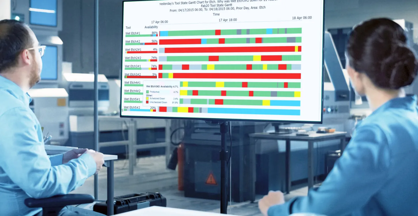
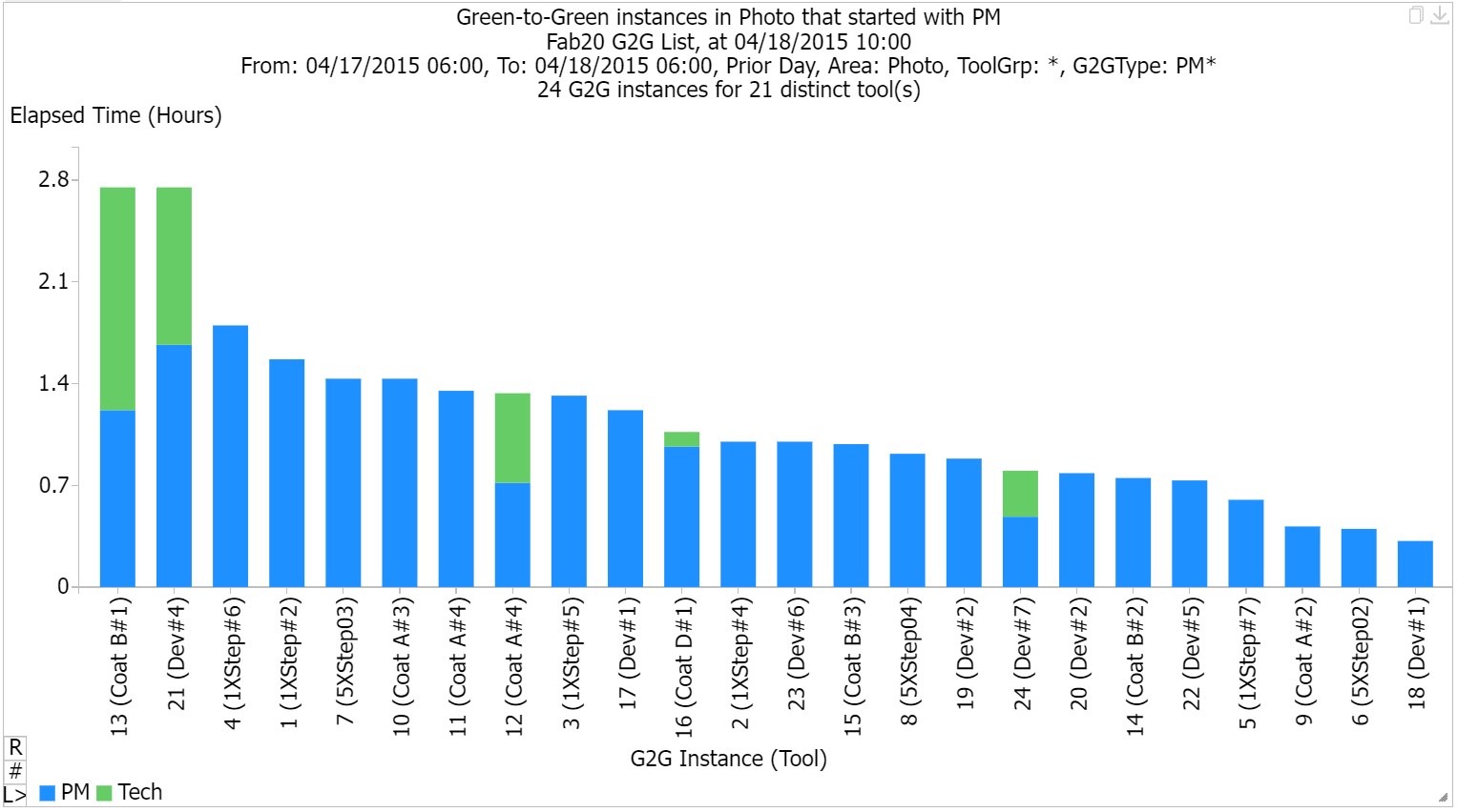
As an example of G2G analysis, we can look at recent PM events in the Photo area, as shown below. Note that the two longest instances are “PM to Repair”. If you group multiple PMs and do them together, they will show up as a longer G2G instance on the above chart. During the instance, the FabTime software ignores transitions to productive, standby, engineering, or nonscheduled time that are less than 2 minutes long (though of course you could select some other threshold). Future enhancements will involve goal setting and trends for G2G instances.

A Few Other Points on PM Tracking and Scheduling
When we wrote about this topic several years ago, we received a detailed response from a longtime subscriber. Here are the highlights.
- The practice of breaking up PM time “is effective for any scheduled event, like changing consumables or performing regularly scheduled tool qualifications when possible.”
- “One of the goals that should be incorporated is to have no scheduled activity last longer than 8 hours. This allows the work to be started and completed on the same shift by the same technician. As many of your subscribers can attest, much time can be lost if the activity crosses over from one technician to another, especially on swing days.”
- “The PM, or any scheduled activity, is composed of work performed when the tool is down (internal) and much more work performed when the tool is running product (external). Things like gathering tools and parts, ensuring any test equipment that may be used is ready, inspecting removed parts, and putting things away are not done when the tool is down.”
The FabTime team agrees with these points, and would also add:
- We believe that this concept can be extended to engineering time. Any time that the tool is unavailable to manufacturing is time during which queue time can build up.
- Although we’re recommending breaking up maintenance events into smaller chunks, instead of grouping them, it’s still true that if you have a fab shutdown, or an extended period when you’re not expecting any WIP to a tool, then you should go ahead and get whatever maintenance you can out of the way. See also the subscriber discussion topic above about dedicating weekends to maintenance.
- Just as it doesn’t make sense to take one tool down for longer than necessary at one time, it also doesn’t make sense to take more than one tool in the same tool group down at the same time, if you have a choice. Staggering maintenance events is much better than doing them simultaneously, so that some amount of WIP continues to get through the tool group. This, we believe, is already common practice in fabs, so we haven’t felt the need to spend much time talking about it here.
Conclusions
There are many sources of variability in wafer fabs, including preventive maintenance events. PM schedules, however, are a relatively controllable knob. Scheduling PMs well can reduce variability in the fab, and thus reduce overall cycle times.
While it can be tempting to group smaller maintenance activities together, or to group them in with other downtime events, this is generally counterproductive for cycle time. What’s best for cycle time is to have each period of unavailable time be as short as possible, particularly for one-of-a-kind tools, to keep lots moving through the tool smoothly. For cycle time, then, it’s better to break PM activity into the smallest possible chunks and make the tool available for production in between.
Clearly, there are limits to this approach, depending on the qualification time required to bring a tool back up, staffing issues, etc. However, it may be worth checking your PM schedules, to see where you may be introducing more variability into the fab than needed. Tracking average and maximum time offline for scheduled downtime, rather than tracking the time between events, is a very good place to start. Even better, we believe, is to use the Green-to-Green metric for capturing the total time that a tool is down, for scheduled and unscheduled downtime, per instance. Using G2G gives you a way to monitor efforts to shorten periods of unavailability, whatever their cause. G2G charts are available in the FabTime reporting module.

