The Three Fundamental Drivers of Fab Cycle Time
Introduction to the three factors that drive wafer fab cycle time at the tool group level: utilization, variability, and number of qualified tools.

At the tool level, utilization, variability, and number of qualified tools are the primary factors that affect cycle time. Other secondary factors such as downtime and setups affect cycle time through their impact on these three primary factors.
Utilization
Utilization has a direct and non-linear impact on cycle times through a tool. Here we define utilization for a tool as the utilization of manufacturing time.
Manufacturing Utilization = Productive Time / (Productive Time + Standby Time)
Productive time is time that the tool is busy processing wafers. Standby time is time that the tool is available, and hence could be processing wafers, but is not. Utilization under this definition is what drives cycle time. In the presence of any variability at all, when standby time gets small relative to productive time, cycle time increases. As standby time approaches zero, cycle time gets very large. Intuitively, what happens is that we need the standby time to recover from variability. When there isn’t much standby time, it takes longer to recover from variability, and cycle times suffer.
For a real-world example, think of driving along on the highway. When there’s not much traffic (utilization is low), you can drive along pretty much unimpeded by other drivers. The more cars there are, however, the more chance there is that someone else will slow you down. If we all drove at exactly the same speed this wouldn’t be so much of an issue. But, of course, we don’t. A gap can form in front of a slower driver, adding a tiny bit of cycle time to the commute time of each and every other driver following behind.
So, we see that as tool utilization increases, cycle times increase. When we graph this behavior (cycle time vs. utilization), we get what’s called an operating curve. An example is shown in the picture below.

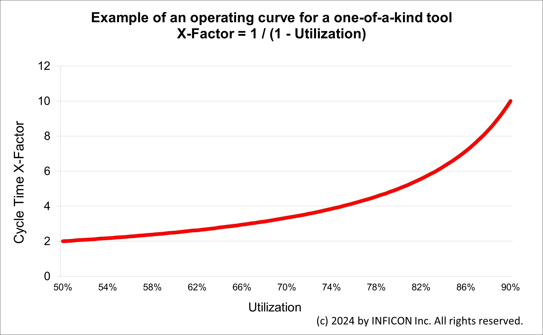
In most cases this operating curve is shaped according to this formula:
Cycle Time X-Factor ~= 1 / ( 1 - Utilization)
Here x-factor is actual cycle time divided by theoretical cycle time. As standby time approaches zero, utilization approaches 100%, and the denominator of the above equation approaches zero. Then we have one divided by zero, which approaches infinity. What we see in practice is that as utilizations get above about 85%, cycle times start to become large. And because the operating curve is non-linear, even small increases in utilization lead to big cycle time increases at this point. This, we believe, is why so many fabs plan capacity such that most tools are loaded to no more than 85%.
For tool groups with only one tool, a moderate amount of variability (exponential process times and times between arrivals), and independent arrival and process times (e.g. the tool does not get faster just because it is busier), the above equation is fairly accurate. It can be used to get a sense for what the cycle time will be for one-of-a-kind tools under different utilization values. For example, if such a one-of-a-kind tool is 75% utilized, then (under moderate variability) the cycle time x-factor is likely to be 1 / ( 1 - 0.75) = 1 / 0.25 = 4 times theoretical.
Utilization is often viewed as relatively fixed on a day to day basis. Fabs are under constant pressure to increase utilization, to make the most of the high capital cost of the equipment. Therefore, saying that you should reduce tool utilization in order to reduce cycle time does not immediately sound practical. However, remember the definition of utilization that we’re using. Productive Time / (Productive Time + Standby Time). The denominator here is also called Manufacturing Time. It’s what you have left after you take out any downtime, engineering time, and non-scheduled time. Therefore, anything that we can do to reduce downtime, engineering time, and non-scheduled time will, if starts are not increased, directly increase standby time. This will reduce utilization, and hence improve cycle time.
One further note is necessary regarding standby time. What drives down cycle time is having standby time as catch-up time on the tool. This means that everywhere that we’ve discussed standby time in the above, we should really be more specific, and refer to standby time during which no WIP is waiting for the tool. This is true standby time. The tool is available, but is not running because there is no WIP waiting to be processed. Having a buffer of such true standby time is helpful for cycle time improvement, because it allows room to recover from variability. If, however, we have time reported as standby time on the tool, during which WIP was qualified and waiting for the tool, this time should really be treated as a loss for the tool. Usually it occurs because there is no operator available to load the tool. Reducing time spent in this state and replacing it with true standby time will improve cycle times.
Variability
Variability also affects cycle times adversely. Variability takes the operating curve of cycle time vs. utilization and moves it upward and to the left. (An example is shown below). This means that for the same utilization, lots passing through higher variability tools will have higher average cycle times. There are many sources of variability in a fab, both in process times and in times between arrivals to tools. Contributors to process time variability include:
- Different recipes on the same machine, with different process times.
- Setups
- Equipment failures and maintenance events
- Rework lots
- Yield loss (scrap)
- Operators
Contributors to variability in arrivals to tools include:
- All of the above (because departures from one step become arrivals to the next step)
- Lot release into the fab
- Transfer batching and automated material handling
- Batch processing (running multiple lots in a machine at one time)

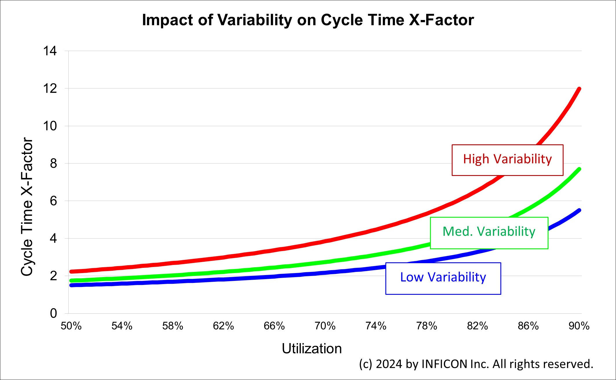
Earlier we said that for a one-of-a-kind tool, the operating curve is shaped like: X-Factor ~= 1 / (1 - Utilization). This was actually a simplification of a more general formula:
X-Factor ~= 1 + [Utilization/(1-Utilization)] * [Variability Factor]
When the variability factor equals one, this reduces to the previous equation (1 / (1 - Utilization)). When the variability factor equals zero, the entire second term drops off, and we get X-Factor ~= 1. That is, we only have cycle time equal to theoretical cycle time when there is no variability. Any variability leads to increased cycle time, particularly when utilization is relatively high. The more variability, the higher the cycle time.
The variability factor is a sum of arrival variability and process time variability. More specifically, the variability factor = (CVa2 + CVp2)/2, where CVa is coefficient of variation of interarrival times, and CVp is coefficient of variation of process times. Coefficient of variation is a statistical measure of how widely dispersed values are, and is equal to standard deviation divided by average. We observe high coefficients of variation when values are widely spread out. For example, arrivals to a tool immediately downstream from a large batch tool might have a high coefficient of variation, because the sequence of times between arrivals looks like this: 0, 0, 0, 0, 0, 0, 0, 0, 12 hours. Here the zeros represent a batch arriving, with essentially no time between arrivals from lot to lot.
In summary, variability in either arrival times or process times increases cycle time. The good news is that anything that you can do to reduce variability will tend to improve cycle times. Some concrete suggestions (which have been discussed in more detail in other newsletter issues) include:
- Reduce transfer batch sizes.
- Eliminate minimum batch size constraints on batch tools that are not heavily loaded.
- Break up maintenance events, to avoid having tools unavailable for long, continuous stretches of time.
- Focus downtime improvement programs on reducing the duration of repair times.
- Spread out lot releases into the fab, instead of releasing lots in large groups.


Free FabTime Operating Curve Generator
Number of Qualified Tools per Tool Group
The third fundamental driver of cycle time at the tool level is tool qualification, or the number of tools available to process a lot at a particular recipe or operation. A recipe with only one qualified tool (often called a single-path tool, or a one-of-a-kind tool) will have higher average cycle times than a recipe with two qualified tools, even if the two tools each have the same utilization as the single tool. A recipe with two qualified tools will have higher cycle times than a recipe with three qualified tools (again, assuming the same utilization on all of the tools), and so on, although the effect is most dramatic when going from one tool to two tools. We have observed that per-visit cycle times are often reduced by about 50% when going from single path to dual path.
For example, suppose that you have two different, equal volume, recipes, which can be run on each of two tools. In the first case, you dedicate each recipe to one of the tools, so that you have two single-path tools. In the second case, you share both recipes across the two tools. The utilization of the tools is the same in both cases. However, the average cycle times through the tools will be approximately twice as high in the first (dedicated) case than in the second (non-dedicated) case. This is because in the dedicated case the single-path tool has less of a buffer against variability. This is often true even if some additional setup/qualification time is needed for the non-dedicated case.

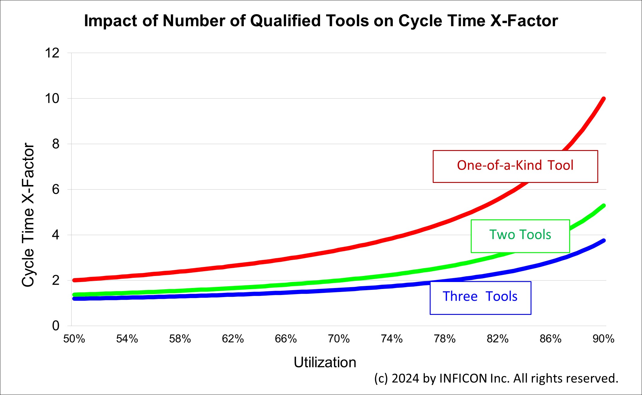
An example is shown above. Cycle time decreases significantly when going from one tool per recipe to two tools per recipe. Cycle time decreases again when going from two tools per recipe to three, but does not decrease by as much.
To think about this intuitively, consider again the example of driving. If you are on a single lane road, and you end up behind a large, slow-moving truck, your cycle time is increased. On a two-lane road you have another lane that you can use to go around the truck. Similarly in the fab, if a single-path tool goes down, or has to process a lot with an exceptionally long process time, everything else has to wait.
What this means is that small fabs with many one-of-a-kind tools will tend to have higher cycle times than large fabs with many similar tools. (This assumes, of course, that the large fab has qualified most of the recipes in the fab to run on multiple tools.) Often this cycle time contribution from one-of-a-kind tools is an inevitable consequence of being a smaller fab. There are, however, sometimes things that can be done to mitigate the problem. Many fabs plan their capacity such that one-of-a-kind tools have a lower planned utilization than other tools (75-80% instead of 85-90%). Focusing variability reduction programs on one-of-a-kind tools can also help, since these tools are the ones most adversely affected by variability.
Another factor to consider is that dedication and qualification policies in many fabs lead to single-path tools, even when other similar tools are available. Sometimes this dedication is necessary, for reasons relating to yield improvement and process restrictions. However, we would urge you to ask your process engineers to re-evaluate tool restrictions from time to time. Sometimes a restriction that is initially put into place can be later relaxed. And the cycle time benefit can be significant. What we have also seen sometimes is what we can “soft constraints.” These occur when operators prefer a certain tool to another, even though both are technically qualified to be used. Searching these out and eliminating them can be a source of cycle time improvement.
Conclusions
In this article, we have reviewed the three fundamental drivers of cycle time: utilization, variability, and number of qualified tools per tool group. Cycle time increases as utilization (Productive Time / (Productive Time + Standby Time)) increases. Anything that can be done to convert non-value-added time such as downtime to standby time (and hence to productive time whenever lots are available for processing) will tend to improve cycle time. Cycle time also increases with variability in process times and in times between arrivals. Variability reduction, then, is a relatively inexpensive way to improve cycle time. Finally, the more tools that are qualified to process each recipe in the fab, the lower the cycle time will be. True one-of-a-kind tools should be planned at lower capacity loading values to improve cycle time, while process restrictions that lead to single-path tools should be examined, and removed where practical. We believe that focusing on these three factors (which interact significantly) will provide an excellent start to any cycle time improvement program.

